


Discover the Very Near Surface
Getting the near-surface right is the difference between a stack that images the subsurface and one that doesn’t.
The problem is right at your feet.
The industry treats the near-surface as a solved problem. The statics say otherwise.
For four decades a quiet contradiction has run through land processing: delay-time statics beat tomostatics, consistently. Tomography produced beautiful models — yet the statics those models implied were almost never as good. If the statics are wrong, the model is wrong.
The reason is the Very Near Surface: a thin, at-the-surface disturbance that contaminates every first break and carries the vast majority of the static. Separate it from the model, and both come out right.
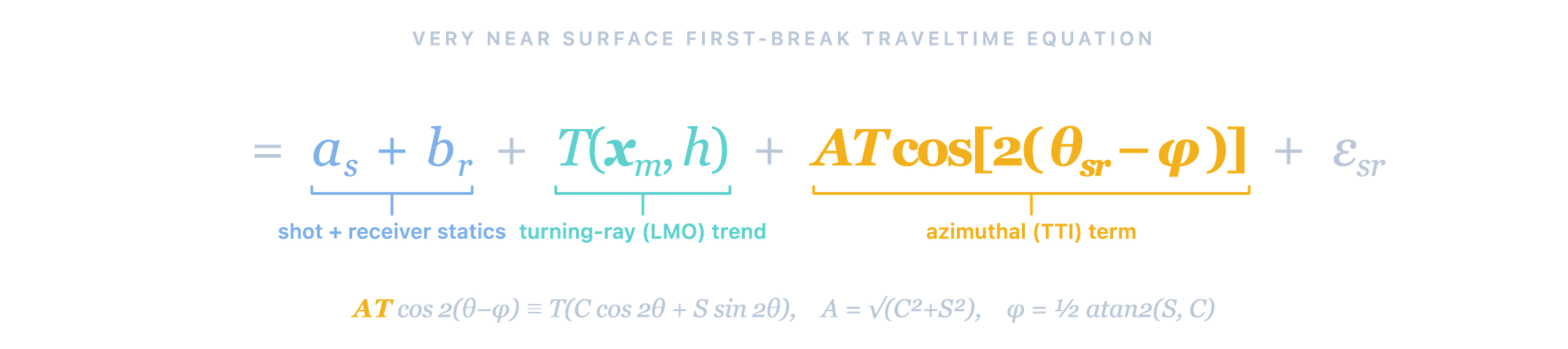
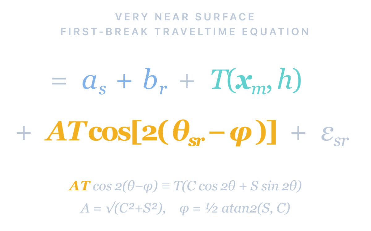
The anisotropic term is TTI — and it is explicit.
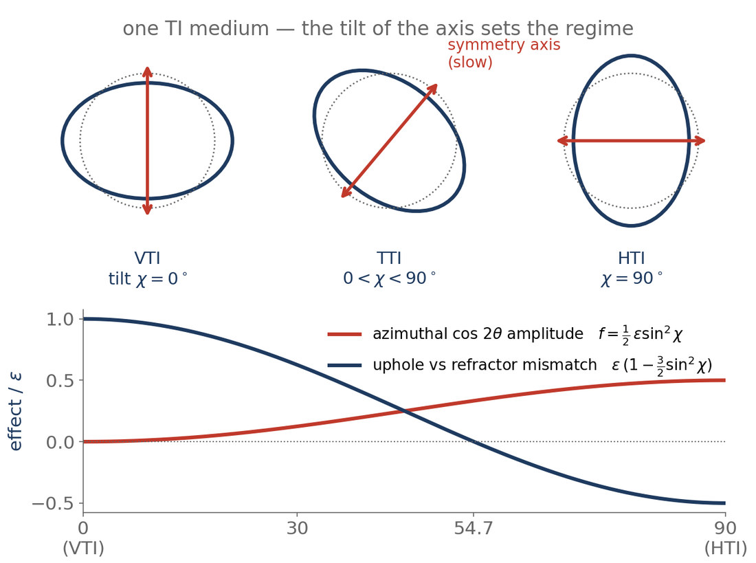
For seismic data in general
Near-surface TTI puts an azimuth- and offset-dependent shift on every arrival — it masquerades as statics plus velocity error, and it degrades stacking, AVO-with-azimuth, and any isotropic model built through it. Because it sits in the first breaks, Sanitas measures it deterministically: a surface-consistent station term (ms) and a per-cell medium term (A, φ) — an explicit field, separable from the data, not an interpretation.
For FWI in particular
FWI’s ability to resolve anisotropy is uncertain — worst in the near surface, where short wavelengths, cycle-skipping risk, and ε–velocity crosstalk collide. An explicit, measured expression for the anisotropy component of the input data changes the problem:
- Correct the data remove the known near-surface anisotropic moveout so FWI does not map it into false shallow structure
- Constrain the model the (vax, εTI, χ, φ) field is a starting/prior TTI model for the shallow section FWI resolves worst
- QC the result FWI-recovered anisotropy has an independent, first-break-measured field to answer to
The near-surface anisotropy stops being FWI’s problem to resolve — it arrives measured.
Rethinking land seismic from the very near surface down.
-
AMGRT · 2025
VNS
First breaks decompose into a surface-consistent shot term, a receiver term, and a turning-ray velocity term. The VNS terms are the statics — they never belonged in the model.
-
2026
Cascade Tomography
An interpretation-free hybrid that separates VNS statics from the tomographic model: delay-time-quality statics and the model you would expect from the surface datum, from a single workflow.
-
2026
Concurrent Anisotropic Tomography
VNS statics, azimuthal anisotropy, and the velocity model solved together — and the anisotropic correction applied through velocity analysis and stack. The first system to close that loop.
The near-surface is the foundation of the house. Every processing step that follows is only as sturdy as what it stands on.
Fix the foundation and the section sharpens.
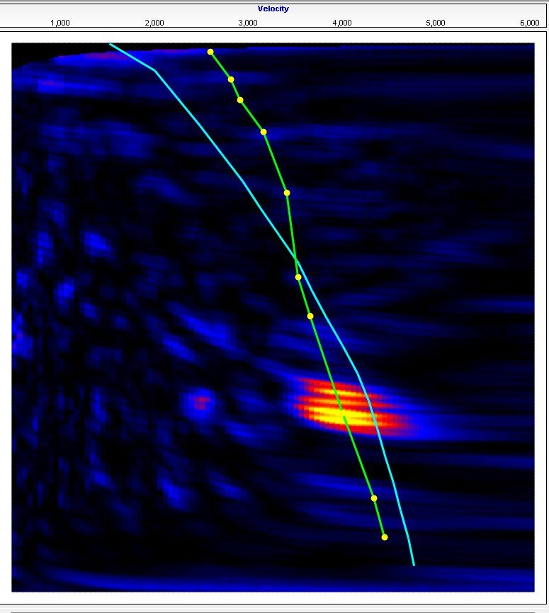
Velocity-analysis semblance on one CMP supergather. With no statics the VNS smears the moveout and the picks are a guess. With Cascade 3-3 and the anisotropy correction the energy collapses into a focused bullseye — before a single processing parameter changed.
2.4×
semblance focus
- No statics
- 0.016
- Cascade 3-3, anisotropy corrected
- 0.039
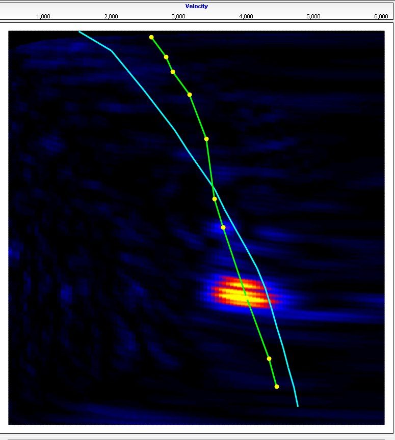
Drag the handle, or focus it and use the arrow keys, to wipe between the two results.
Stack, Profile 1
Cascade 3-3 statics, anisotropy applied. Reflector continuity restored end to end — no smoothing, no interpretation, no hand-editing.


Drag the handle, or focus it and use the arrow keys, to wipe between the two results.
The senior processor’s route — and the senior processor’s reasoning.
Any Sanitas workflow can be captured as a Trail: a guided sequence of the system’s own working windows — pick the trends, build the model, compute the statics, QC the stack — each step pared to its task, presented in order, branching where a decision changes the path.
Embedded in every Trail is SeisMentor™: ask why at any step and get answers grounded in the CT-VNS methodology and your project’s own numbers.
Experts author Trails; the library ships with the system; the expertise that usually lives in one person’s head becomes something the whole shop runs.

One system, end to end
Sanitas is the newest life of a processing engine with a two-decade commercial pedigree in refraction statics — rebuilt around VNS, and carrying the correction all the way through velocity analysis and stack.
-
Sanitas
Eikonal tomography, cascade passes and concurrent azimuthal anisotropy in one processing system.
-
Guided workflows
Any workflow can be captured as a guided sequence of the system’s own working windows, in order, branching where a decision changes the path.
-
SeisMentor™
Ask why at any step and get answers grounded in the CT-VNS methodology and your project’s own numbers.
The Best bring us their Worst.
Start with the near-surface: read the full guide to both statics pathways, or bring us a dataset and talk it through with the people who built the system.
SEG IMAGE 2026 · Houston Booth 846 Live demos daily