Traditional Refraction and Turning-ray Tomography Statics
Delay-time & turning-ray tomographic workflows for conventional near-surface conditions.


From conventional delay-time analysis to cascade anisotropic tomography.
Getting the near-surface right is the difference between a stack that images the subsurface and one that doesn’t. Sanitas offers two statics pathways — the Traditional Refraction Statics, and the Cascade Anisotropic Tomography built for complex, azimuthally-varying near-surface conditions.
Delay-time & turning-ray tomographic workflows for conventional near-surface conditions.
Multi-pass eikonal tomography with anisotropic correction for complex near-surface geology.
Conventional delay-time analysis and turning-ray tomography, inside Sanitas. Traditional refraction statics starts with first breaks picked across multiple planes, then follows one of two proven paths to a near-surface correction.

Assign first breaks to refractors, run refraction analysis (refractor velocity + delay times), build the refractor model, and estimate statics directly.
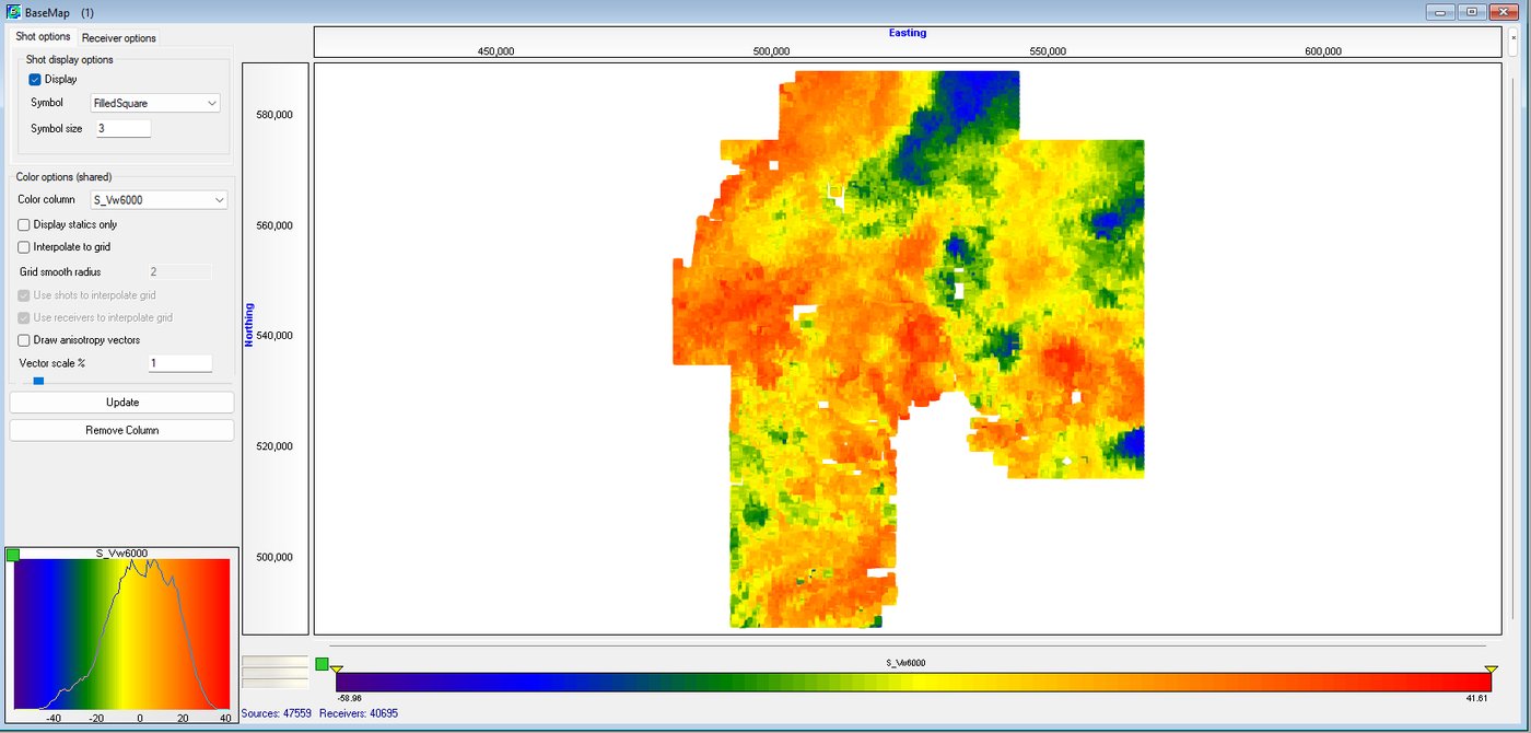
Define an initial tomographic model (velocity range, max depth), select reliable offsets, and iteratively build a turning-ray tomographic model.
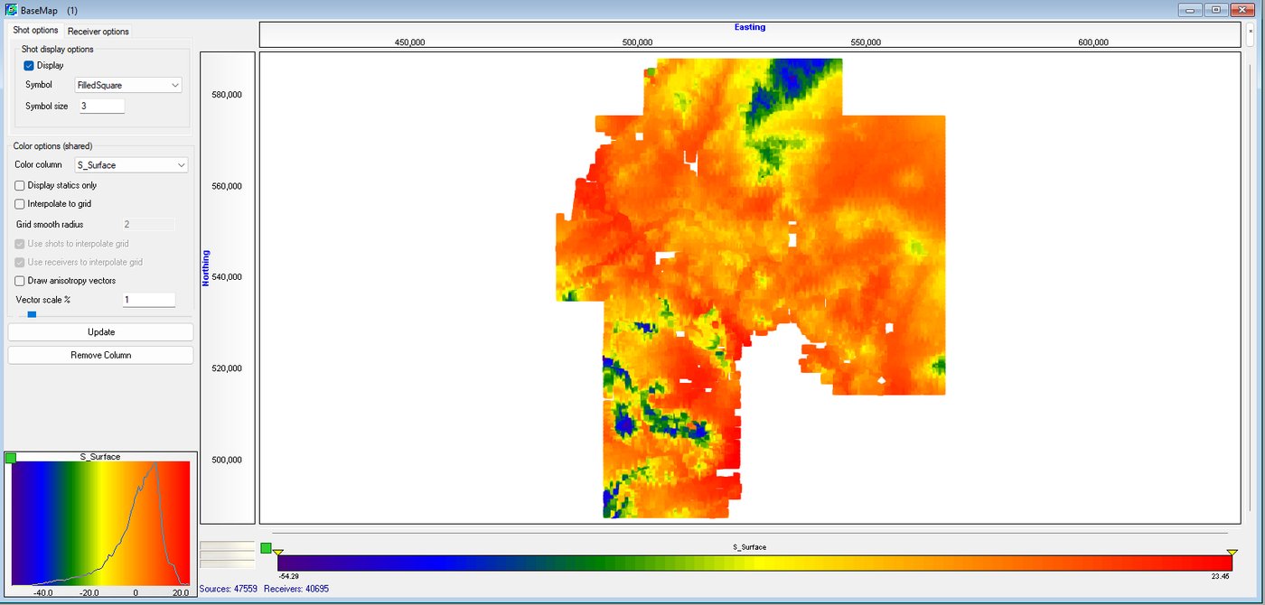
First breaks picked across multiple planes.
Refractor velocity and delay times.
Build the refractor or tomographic model.
Estimate the near-surface correction.
Multi-pass eikonal tomography built for azimuthally complex near-surface geology. Also referred to in the source material as Cascade Anisotropic Tomographic Statics.
Where a single tomographic pass falls short, Sanitas runs Eikonal tomography in cascade — multiple successive passes — combined with anisotropic analysis.
A first-of-its-kind workflow: statics AND anisotropic correction applied to both velocity analysis and the final stack, solving a problem no other land processing system addresses.
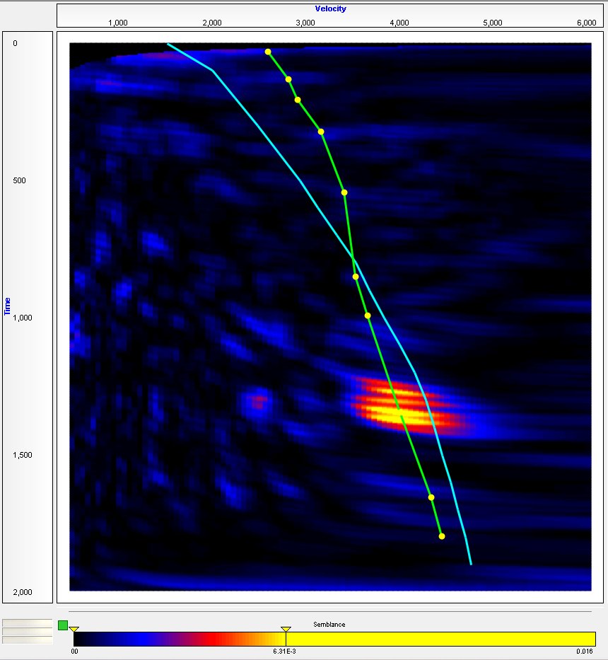
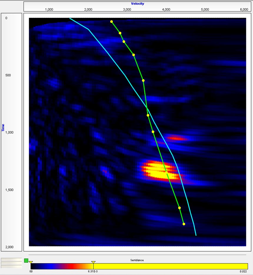
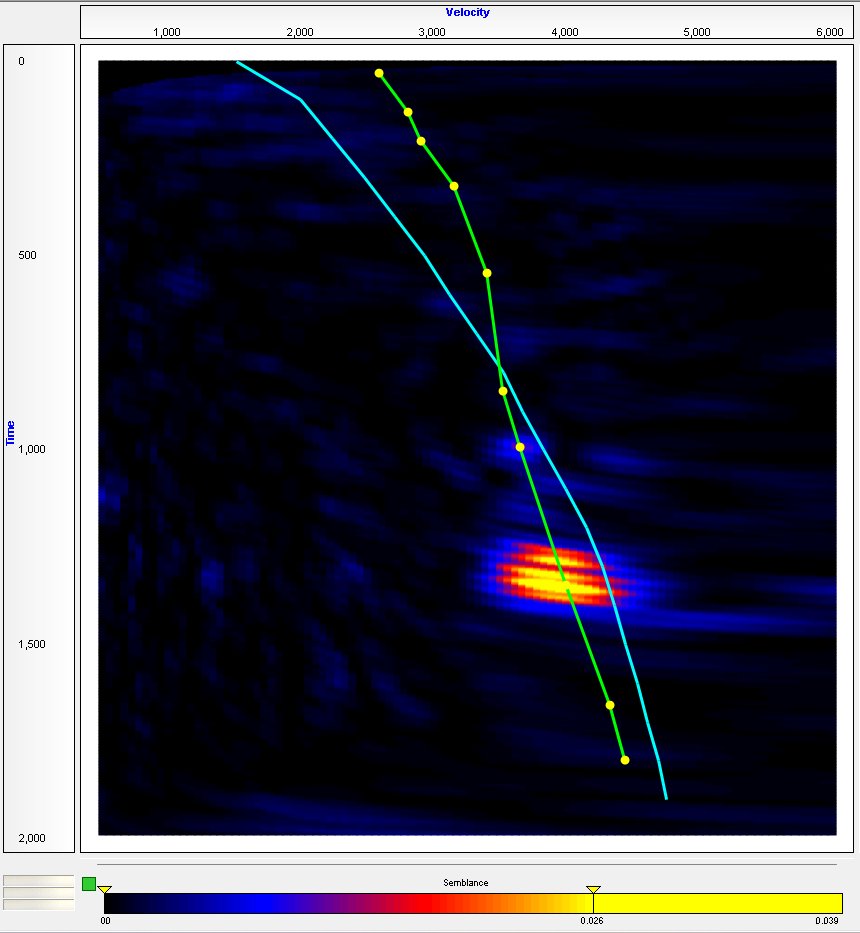


A side-by-side comparison of the two pathways.
| Attribute | Traditional Refraction Statics | Cascade Anisotropic Tomography |
|---|---|---|
| Core method | Traditional Refraction Statics Delay-time analysis or single-pass turning-ray tomography | Cascade Anisotropic Tomography Multi-pass (cascade) Eikonal tomography |
| Anisotropy | Traditional Refraction Statics Not modeled | Cascade Anisotropic Tomography Explicitly analyzed and corrected |
| Best suited for | Traditional Refraction Statics Conventional, laterally consistent near-surface | Cascade Anisotropic Tomography Complex, azimuthally-varying near-surface |
| Applied to | Traditional Refraction Statics Statics only | Cascade Anisotropic Tomography Statics and anisotropic correction, on both velocity analysis and stacks |
| Guided by | Traditional Refraction Statics Sanitas TrailMap: Trend → Tomo | Cascade Anisotropic Tomography Sanitas TrailMap: Trend → Cascade (with anisotropy) |
The Sanitas TrailMap is an interactive tutor that carries you through the exact sequence of live, functioning Sanitas windows needed to reach a specific goal, using your own active project.
Pre-built trail maps cover both paths in this guide, including Trend→Tomo, Trend→Cascade, and their anisotropy-aware variants.

Any Sanitas workflow can be captured as a Trail: a guided sequence of the system’s own working windows — pick the trends, build the model, compute the statics, QC the stack — each step pared to its task, presented in order, branching where a decision changes the path.
Embedded in every Trail is SeisMentor: ask why at any step and get answers grounded in the CT-VNS methodology and your project’s own numbers.
Both statics pathways in one guide — traditional refraction statics, cascade anisotropic tomography, the comparison table, and Sanitas TrailMap. PDF, 4 pages.
Bring us a dataset and talk it through with the people who built the system.